CHAPTER III To work with Powersim Study: introduction to I use it of the software through a practical example.
3.15 To carry out an execution of test of the model
Powersim contains a called commando “Report Car” that concurs to examine the behavior and the value of the variable ones
in the diagram.
Since the orders increase after twenty weeks, expect to see a decrease to us in the inventory after this period of time.
In order to see this decrease better the function “Time can be used graph Report Car exactly”.
- Cliccare with the skillful key of the mouse on the variable “Inventory” and to select Show Report Car and in sottomenu Time Graph Report Car;
- Ciccare Play in order to execute the simulation.
The development of the inventory will be shown in the Report Car.
To the end of the simulation the shown situation of continuation will be had.
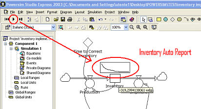
Figure 3.13- After 20 weeks the inventory will begin to decrease. To the end of the simulation an inventory will be had negative from the moment that the production is not increased in order to compensate greater shipments.
As it can be seen from the figure the inventory is diminished assuming a value negative.
Given the new rate entering orders, that is not amazing, in how much the value of the shipments (Shipments) is greater
of that one of the production through the greater part of the simulation.
This has had to the fact that the variable “Desired Inventory” not rispecchia the variation of the question that verification
after twenty weeks.
In order to implement a sensibility to the question waited for Question must introduce the concept of “Expected Demand” ().
3.16 To add the concept of waited for question
Expected demand is an important leaves of this model because it translate the variations of the question in production variations.
That is it takes to the information from the market (Order Installments) and it converts to them in actions that control the amount to produce.
The question is not a physical accumulation like the inventory. However the represented accumulations the levels do not have
necessarily to be physical accumulations.
Since there is need to introduce a delay in the changes of the attended question, the better way than to model
“Expected Demand” it is under level shape.
- To create a Level in the model and rinominarlo “Expected Demand”;
- To define it with a value begins them of 100<> that he is equal to the rate it begins them of entering orders.
The Flows are the only elements that can change the levels, therefore are need of a flow in order to represent
the variation of “Expected Demand”.
There is also need of a factor of time in order to indicate how much time serves in order to change the question attended in real question.
- To create a new flow that enters in the level “Expected Demand”;
- Rinominare the new flow in “Change in Expected Demand”;
- To add one constant name “Time to Change Expectations”;
- To connect “Order Installments”, “Expected Demand” and “Time to Change Expectations” to the flow “Change in Expected Demand”.
Variable “Time to Change Expectation” represents the time necessary in order to correct the waits on the question in real
question.
This is one constant and par to eight weeks is assumed (8< < wk> >); the variable “Ch'ange in Expected defined Demand” like:
“(“Order Installments” - “Expected Demand”)/“Time to Change Expectations””.
The model hour contains one structure in order to estimate the question attended in the market (figure 3.14).
It depends on the rate running order and the constant of time.
This constant of time represents the time that is necessary to the society in order to change its opinion on the question in the market.
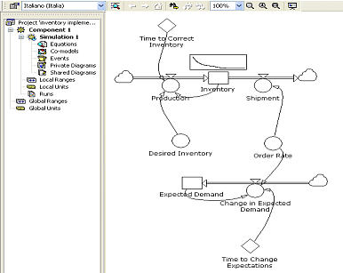
Figure 3.14- The model hour contains one structure in order to find the question waited for (Expected Demand)