CHAPTER III To work with Powersim Study: introduction to I use it of the software through a practical example.
3.19 To compare “Inventory” and “Desired Inventory”
To create an other diagram of time in which inserting variable “the Inventory” and “Desired Inventory”.
The diagram of the new simulation is shown in figure 3.17:
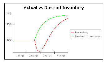
Figure 3.17- The graphical extension the inventory puts into effect them and that one wished. Desired Inventory grows immediately when the orders increase, but because of the delay in the production the inventory decreases before catching up the same level of “Desired Inventory”.
3.20 Behavior of the model
For the first twenty weeks of the simulation all the variable ones are constant and that indicates that the model is in equilibrium.
After twenty weeks the model goes outside the equilibrium because of the variable “Order Installments” that door from hundreds to
centoventi widgets to week for all the rest of the simulation.
This behavior constitutes a shock for the model and reveals its dynamic behavior.
It turns out you of the “shock” can have had to the behavior of the other variable ones.
“Expected Demand” can increase, but slowly, end when it catches up the new level of the entering orders.
The rate with which it increases is slow in how much the flow changes to the question attended second the discrepancy between
“Order Installments” and “Expected Demand”. This discrepancy is larger when the “shock” happens.
From this moment “Expected Demand” it grows gradually reducing such discrepancy.
“Production” grows above “Order Installments” before ring-establish the equilibrium.
“Desired Inventory” grows anch'esso (increasing the difference between “Desired Inventory” and “Inventory”) because it is simply
a multiple of “Expected Demand”.
The increase of the production is also obvious from the behavior of the inventory. In this society the shipments are always
equal to the order rate so that the increase of shipments begins to cause the emptying of the inventory.
This increases to the discrepancy between the wished inventory and that real one. When the production catches up the rate orders,
the inventory catches up its minimal level.
This happens approximately after 25 weeks. From in then the production it goes here to of over of shipments allowing
to the inventory increasing.
After 25 weeks, therefore, as the difference between “Desired Inventory” and “Inventory” is closed and the waited for question catches up
the orders, the production decreases until the attainment of the equilibrium.
After approximately 70 weeks the model it is of new in equilibrium.
This thing means in terms of market operations? The beauty to create a model of a system is that one
to allow us to not only investigate on the structure of a system (like levels and flows are appropriate to you) but also
as changes on the structure change the behavior of the system (in this case consider the performances
of the system).